Anisotropy and Volume Fraction Mapping of a Proximal Femur
This Bone Analysis tutorial provides step-by-step instructions for segmenting a proximal femur and for computing vector-based fields of anisotropy and scalar-based maps of volume fraction. Additional topics in this tutorial describe how to compute high-resolution maps from data sub-volumes and how to evaluate the computed maps.
Screen capture of the completed tutorial

Before you start the tutorial, you should download and unzip the tutorial dataset — Proximal Femur. This dataset, as well as the session file of the tutorial, are available on the ORS website at: http://www.theobjects.com/dragonfly/learn-sample-datasets.html.
In this section, you will learn how to extract the required region of interest from a threshold range. Instructions for refining the initial segmentation are also included here.
- Load the tutorial dataset or a similar sample (see Importing Image Files).
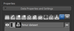
The dataset appears in the Data Properties and Settings panel.
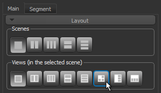
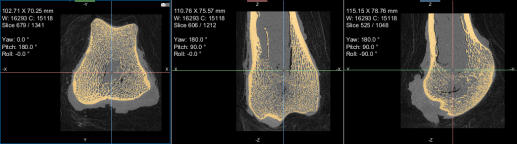
- Display the data in a 2x2 layout by clicking the Views icon, as shown below.
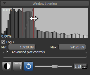
- Adjust window leveling, as required (see Window Leveling).
- In 3D views, it is often best to adjust window leveling on the histogram, as shown below.
- In 2D views, it is often quickest to use the Area
 tool to adjust leveling, as shown below.

- In 3D views, it is often best to adjust window leveling on the histogram, as shown below.
- Create a region of interest with data values thresholded for mineralized bone as follows:
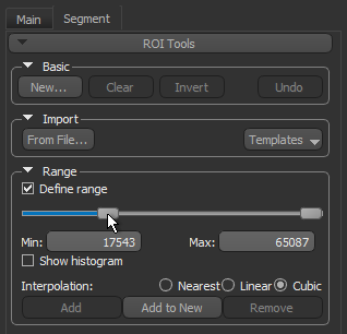
- Click the Segment tab on the left sidebar to access the ROI Tools panel.
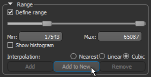
- Select the Define range option in the Range box on the ROI Tools panel.
- Drag the left or right Range sliders to change the minimum or maximum values of the intensity range or enter the required values in the Min and Max edit boxes.
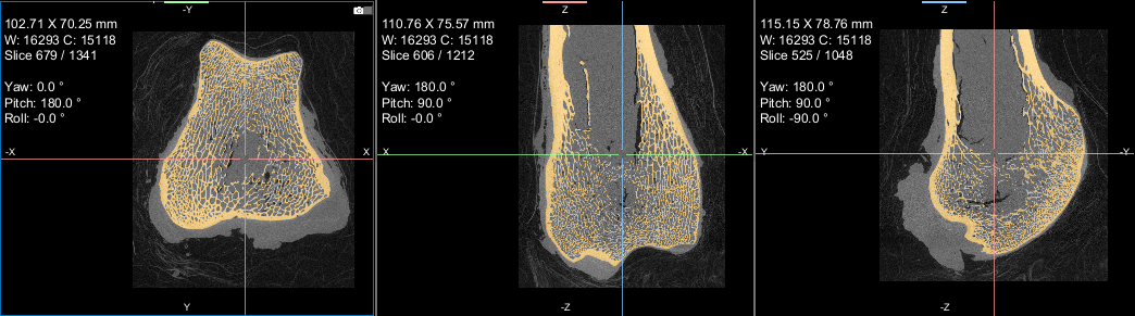
- Verify the selected range on other images in the image stack and other views of the dataset, recommended.
- Click the Add to New button to create a region of interest in which all voxels within the selected range are labeled.
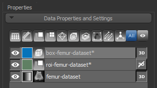
A new region of interest is added to the Data Properties and Settings panel. Information about the new ROI is displayed in the lower section of the Data Properties and Settings (see ROI Properties and Settings).
- Uncheck the Define range option in the Range box.
- Remove noise and other unwanted objects from the region of interest as follows:
- Right-click the region of interest in the Data Properties and Settings panel and then choose Process Islands > Isolate (6-connected) nth First Biggest in the pop-up menu.
- Enter 1 in the Isolate Biggest Count dialog and then click the OK button.
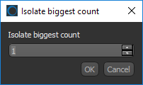
All unconnected objects that are smaller than the largest object in the region of interest are removed from the ROI (see Processing Islands for more information about this feature).
NOTE With this initial bone segmentation you can separate the cortical shell from the trabecular interior automatically and then compute morphometric indices (see Computing Cortical and Trabecular Measurements).
- Continue to the next section to learn how to compute 3D vector field-based maps of anisotropy.

This section provides step-by-step instructions for computing a 3D vector field-based map of anisotropy.
- Make sure that the required region of interest is selected in the Data Properties and Settings panel.
- Create a box that either entirely or partially encloses the region of interest as follows:
- Click the Box button in the Shapes panel.
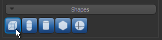
A new Box shape appears in the Data Properties and Settings panel. Click the Eye icon to show the box in the workspace views.
- Adjust the box in the 2D and/or 3D views of the region of interest, as required.
You can resize and rotate the box, as well as change its position with the available control points (see Editing Shapes).

- Click the Box button in the Shapes panel.
- Choose Tools > Bone Analysis on the menu bar to open the Bone Analysis dialog.
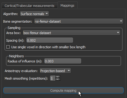
- Do the following on the Mappings tab:
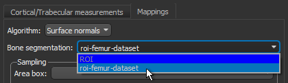
- Choose Surface normals in the Algorithm drop-down menu.
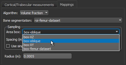
- Choose the region of interest that you created for this tutorial in the Bone segmentation drop-down menu.
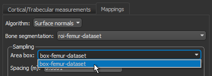
- Choose the box that encloses the area that you want to include in your analysis in the Area box drop-down menu.
- Enter a value of 0.002 m in the Spacing edit box.
NOTE Although the highest resolution, or lowest spacing, of the tutorial dataset is 0.5 mm, this should be increased to 2.0 mm if the entire 3D shape of the femur will be mapped.
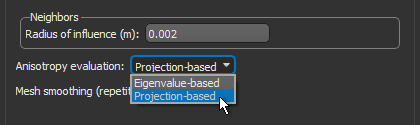
- Select a value between 1 and 3 mm in the Radius of influence edit box.
NOTE The radius of influence defines the kernel size, or elementary volume, within which anisotropy will be evaluated. You should note that a too small radius of influence may result in a low signal-to-noise ratio, while a too high radius can result in averaging and edge effects.
- Choose Projection-based in the Anisotropy drop-down menu.
- Choose a number of iterations in the Mesh smoothing (repetitions) spin box, optional.
- Click the Compute Mapping button.
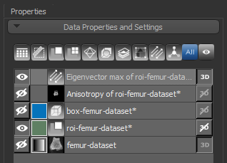
Two new items — a vector field and scalar-based anisotropy dataset — appear in the Data Properties and Settings panel after all computations are complete.
- Continue to the next section to learn how to examine the vector field-based map.

This section describes the different settings that can be applied to the vector field-based anisotropy map that was computed in this tutorial.
Below are some examples of vector field-based anisotropy maps shown from different aspects. The top row includes visualizations of anisotropy magnitude, while the bottom row shows vector fields colored by orientation. The pair of images on the right show maps that are clipped.


- Maximize the 3D view in the workspace, recommended.
- You can maximize a view by double-clicking it or you can right-click and then choose Maximize View in the pop-up menu.
- Select the 3D vector map you created and make it visible in the 3D view by clicking the Eye icon in the Data Properties and Settings panel.
The 3D vector field-based anisotropy map appears in the 3D view at the default settings, with the vectors corresponding to the highest surface anisotropy colored yellow and those corresponding to the lowest, or isotropy, colored blue.

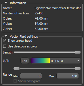
Information and settings related to the selected vector-based field appear in the bottom section of the Data Properties and Settings panel.
NOTE In most cases, you should hide the rendering of the dataset if it is visible in the 3D view.
- Change the settings applied to the 3D vector field-based map, as described below.
- Uncheck the Show arrow head option. This usually improves the visibility of the vectors in the field.

- Use the Length slider to adjust the length of the vectors.
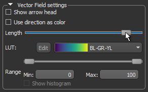
- Choose another look-up table (LUT) in the LUT drop-down menu.
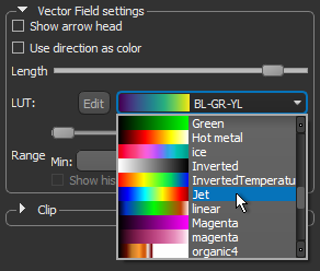
NOTE The Jet LUT is often a good color scheme choice. In this LUT, vectors corresponding to the highest surface anisotropy are colored red, while those corresponding to the lowest, or are isotropic, are colored blue.

- Threshold the vector field-based map to show only high or low anisotropy areas with the Range slider, as shown below.
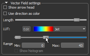
The thresholded map shown below shows only low anisotropy areas located near articulating surfaces.

- Check the Use direction as color option.
Checking this option will re-code the vector map in accordance with the orientation of the vectors — red for the X axis, green for the Y axis, and blue for the Z axis.

- Apply clipping to evaluate inner surfaces (see Clipping).
- Uncheck the Show arrow head option. This usually improves the visibility of the vectors in the field.
- Continue to the next section to learn how to create high-resolution anisotropy maps in different orientations.


This section of the proximal femur tutorial describes how to compute high-resolution anisotropy maps in different orientations. You should note that when computing high-resolution maps, you should limit the volume of operation to regions that enclose only part of the region of interest. This can be done by creating a series of boxes that describe a particular orientation.
The images below (from left to right) correspond to XZ, XY, and oblique orientations. The computed vector fields are colored by magnitude.
High-definition vector field-based surface anisotropy maps

- Create a series boxes to enclose parts of the original region of interest.
You can resize and rotate the boxes, as well as change their position within a 2D or 3D view with the control points (see Editing Shapes).
- Adjust the boxes as follows:
- Drag any face of the box to resize it, as shown below.

- Drag a control point to resize and/or rotate the box, as shown below. You can also translate a box by dragging from its central control point.

- Drag any face of the box to resize it, as shown below.
- Choose the settings for each high-definition vector field-based surface anisotropy maps on the Mappings tab, as shown below.

NOTE You can decrease the sampling spacing and radius of influence to 0.0005 m and 0.0015 m, respectively, since you will be computing maps within a sub-volume.
- Click the Compute mapping button.
- Examine the results (see Examining the Computed Vector Field-Based Map).


This section of the tutorial describes how to use the Bone Analysis module for 3D volume fraction plotting. You should note that volume fractions are scalar maps.
Comparison of volume fraction scalar map (on left) with vector-based field of anisotropy (on right)

- Create additional boxes to enclose different parts of the original region of interest, if required.
NOTE You can also use any of the boxes you created previously in this tutorial to map volume fraction.
- Choose the settings for the volume fraction map on the Mappings tab, as shown below.
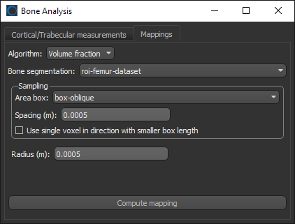
- Click the Compute mapping button.
When processing is complete, the volume fraction dataset appears on the Data Properties and Settings panel.
- Examine the volume fraction map in the 3D or 2D views in the workspace.

NOTE In most cases, the Jet LUT provides good visualizations of volume fraction.


