Computing and Visualizing Mappings of Anisotropy and Volume Fraction
Computing and mapping surface and volume anisotropy by magnitude and orientation as vector fields and volume fraction as scalar values can help identify heterogeneity and latent features to correlate form with function in bone specimens. The options for computing anisotropy maps with the MIL and Surface normals algorithms, as well as for computing volume fraction, are available in the Bone Analysis dialog. Visualizations of vector-based maps are available in the 3D views in the workspace, while the mapped scalar values of volume fractions can be examined in both 2D and 3D views.
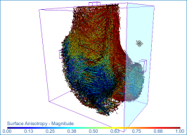
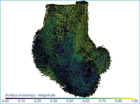
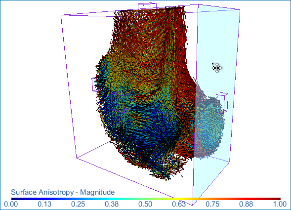
Surface anisotropy magnitude (left) and orientation (middle) and volume fraction (right) of a proximal femur

Two mapping methods — MIL and Surface normals — are available in the Bone Analysis module for computing anisotropy, as well as the option to generate scalar-based maps of volume fraction. These mapping methods are described below.
MIL… This classic method of anisotropy measurement using the Mean Intercept Length (MIL) method combines both surface and volume anisotropy components and requires sampling volumes to be about 4-5 inter-trabecular spaces.
Surface normals… The surface anisotropy measurement exclusive to Dragonfly is based on the construction of a surface mesh populated by a set of vectors perpendicular to the mesh faces with their magnitude being proportional to the local mesh face area. For each anisotropy evaluation point, the faces having their center at a distance smaller than the radius of influence are identified. A tensor of inertia is constructed using the normals of these faces, linearly weighted by their area and weighted on their distance to the evaluation point by the function: w(d) = 1 - (d2)/(r_max2). The eigenvectors and eigenvalues of the tensor of inertia are obtained. The eigenvector corresponding to the greatest eigenvalue, corresponding to the smallest moment of inertia (maximal elongation) is taken as the anisotropy orientation.
The Projection-based algorithm computes anisotropy as:
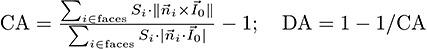
, where CA is the coefficient of anisotropy, S is the local mesh face area, n is the normal to the face, IO is the anisotropy orientation, DA is the degree of anisotropy. DA is a measure of how highly oriented substructures are within a volume. For an isotropic (perfectly oriented) system, the degree of anisotropy is equal to 0. As the system becomes more anisotropic (less well-oriented), the DA increases to some value less than or equal to 1.
The Eigenvalue-based algorithm gets anisotropy from the eigenvalues of the tensor of inertia, which is similar to the MIL algorithm.
The surface normals algorithm can provide very good general orientation information as well as high-resolution anisotropy values. For computations with the surface normals algorithm, the radius of influence can be as small as the size of a single trabeculae.
Volume fraction… The computed output is the proportion of the sample volume that is mineralized bone, in which a scalar value — 1 for high and 0 for low — is assigned to every spatial position (labeled voxel) in the input region of interest.
The global settings for computing mappings are described in the table below.
|
|
Description |
|---|---|
|
Area box |
Defines the analysis area for computing the selected mapping RECOMMENDATIONS In cases in which you need very precise measurements and plan to use a small spacing value, you should reduce the area box as much as possible. You can also add multiple boxes to compute anisotropy and volume fraction maps in different orientations. |
|
Spacing |
Determines the distance between the random points in the analysis area Use single voxel in direction with smaller box length… If checked, computations will limited to a single voxel in the direction of the smallest length of the selected area box
|

The settings available for each mapping method are described in the table below.
The settings for the MIL algorithm are listed in the table below.
|
|
Description |
|---|---|
|
Sampling |
The resolution, or distance between subsequent samples along each vector RECOMMENDATIONS The entered value should be about 4-5 inter-trabecular spaces. |
|
Radius |
The radius of the sampling sphere, which determines the length of each sampling vector |
|
Orientations |
The number of lines to analyze per sampling sphere |
The settings for the Surface normals algorithm are listed in the table below.
|
|
Description |
|---|---|
|
Neighors |
The Radius of Influence defines the kernel size, or elementary volume, within which anisotropy will be evaluated RECOMMENDATIONS The radius of influence can be as small as the size of a single trabeculae. |
|
Anisotropy evaluation |
Lets you choose an anisotropy evaluation method — Projection-based or Eigenvalue-based. You should note that both methods provide similar results, although you may find that the Projection-based method is slightly more sensitive. |
|
Mesh smoothing (repetitions) |
Determines number of times that the mesh obtained from the input ROI will be smoothed before computing anisotropy RECOMMENDATIONS Selecting one or two iterations of smoothing usually provides for the most accurate result. |
The settings for the Volume fraction algorithm are listed in the table below.
|
|
Description |
|---|---|
|
Radius |
The distance from the analysis point to the last considered ROI element |
Mappings of anisotropy and volume fraction can be computed from bone segmentations within the area defined by a Box shape. The inputs can be any region of interest or mesh, while the outputs of anisotropy and volume fraction mapping computations include the following:
Anisotropy of… Scalar-based map of anisotropy (channelAnisotropyMapping).
Eigenvector max of… Orientation field of the eigenvector associated to the highest eigenvalue (vectorFieldEigenvectorMax).
Volume fraction of… Scalar-based map of volume fraction (channelVolumeFractionMapping).
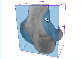
- Add a Box shape to the workspace and size it to the region in which you want to compute the required mapping as follows:
- Select the region of interest that will be the input for computing the mapping in the Data Properties and Settings panel, recommended.
- Click the Box
 shape in the Shapes panel.
 - Make the shape visible by clicking its associated Eye icon in the Data Properties and Settings panel.
- Adjust the size and position of the shape, as required (see Editing Shapes for information about resizing, rotating, and repositioning shapes).
NOTE In cases in which you need very precise measurements and plan to use a small spacing value, you should reduce the box as much as possible. You can also add multiple boxes to compute anisotropy and volume fraction maps in different orientations.
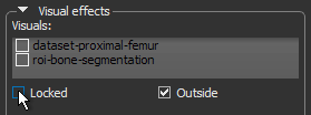
- Lock the shape by checking the Locked option in the Visual effects box, recommended.
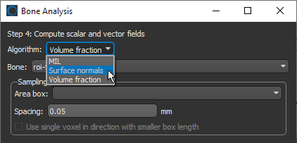
- Choose Tools > Bone Analysis on the menu bar to open the Bone Analysis dialog.
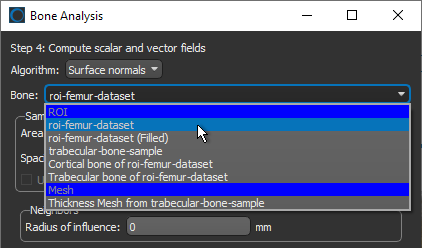
- Navigate to the Compute scalar and vector fields screen by clicking the Next button at the bottom of the dialog.
- Select a mapping method in the Algorithm drop-down menu (see Mappings Methods and Settings).
- Select the region of interest or mesh that you want to map in the Bone drop-down menu.
- Select the Box shape that defines the region in which you want to compute the mapping in the Area box drop-down menu.
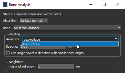
- Enter the required spacing value in the Spacing edit box (see Global Settings).
NOTE For faster computations, and to obtain orientation fields that are easier to observe, you can select the Use single voxel in direction with smaller box length option. In this case, computations will limited to a single voxel in the direction of the smallest length of the selected area box.
- Enter the required settings for the selected algorithm (see Algorithm Settings).
- Click the Compute scalar and vector fields button to start the computation.
This will map the anisotropy of 3D surfaces — their preferred orientation and the direction of that preferred orientation with respect to the Cartesian coordinates — or the volume fraction.
At the end of the process, the requested vector field and/or generated dataset will appear in the Data Properties and Settings panel.
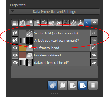
- Continue to the next section to learn how to view vector fields and mappings of volume fraction.
Visualizations of vector-based maps are available in the 3D views in the workspace (see Visualizing Vector-Based Maps of Anisotropy), while the scalar-based maps of volume fraction datasets can be evaluated in 2D and 3D views (see Visualizing Volume Fractions).
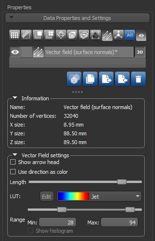
Settings for visualizing vector-based maps in 3D views, as well as basic information about a selected object, are available in the Data Properties and Settings panel, shown below.
Vector field properties and settings
|
|
Description |
|---|---|
|
Name |
Indicates the name of the selected vector field. |
|
Number of vertices |
Indicates the total number of vertices in the computed surface mesh. |
|
X size |
indicates the dimension of the selected vector field in the X axis. |
|
Y size |
indicates the dimension of the selected vector field in the Y axis. |
|
Z size |
indicates the dimension of the selected vector field in the Z axis. |
The following settings are available for adjusting visualizations of vector fields.
|
|
Description |
|---|---|
|
Show arrow head |
If selected, arrow heads will appear on each vector in the field. |
|
Use direction as color |
If selected, each Euclidean vector will be colored according to its orientation — X in red, Y in green, and Z in blue. If not selected, each Euclidean vector will be colored according to the anisotropy value computed in the output anisotropy dataset. Coloring is selectable in the LUT drop-down menu. |
|
Length slider |
Lets you adjust the length of the Euclidean vectors in the selected vector field. |
|
LUT |
Lets you select the colors that will be applied to mapped anisotropy values. NOTE This option is not available whenever the Use direction as color option is selected. |
|
Range |
Lets you threshold the minimum and maximum values that are displayed. |
- Select a 3D view in the workspace.
- Select the required vector field in the Data Properties and Settings panel.
Information and settings related to the selected vector field appear below the listed items in the Data Properties and Settings panel.
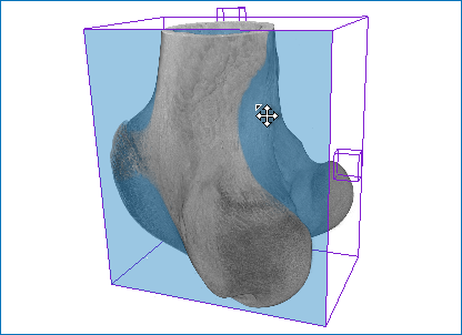
- Make the vector field visible by clicking the Eye icon.
The vector field appears in the 3D view at the default settings, in which each vector is colored according to the anisotropy value computed in the output dataset.

- Adjust the settings in the Vector field settings box, as required.
- You can uncheck the Show arrow head option to improve the visibility of the vectors in the field.
- You can adjust the length of the vectors, as well as select a different color mapping scheme in the LUT drop-down menu.
- You can threshold the minimum and maximum values that are displayed with the Range sliders or by entered new values in the Min and Max range boxes.
- You can color each vector according to its orientation by checking the Use direction as color option. If this option is selected, vectors oriented in the X axis will be colored red, vectors oriented in the Y axis will be colored green, and those oriented in the Z axis will be colored blue.
NOTE See 3D Scene's View Properties for information about adjusting the properties of the 3D scene view.
- Apply clipping, if required (see Clipping).
To clip a vector field, click the Clip
 tool on the Clip panel and then do the following:
- Drag a face of the Clip box to move a plane up and down or in and out. Each plane of the 6 sides of the parallelogram can be moved independently.
- Drag any of the control points to rotate a side of the parallelogram.
- Translate the Clip box by dragging from the central control point.
- Drag a face of the Clip box to move a plane up and down or in and out. Each plane of the 6 sides of the parallelogram can be moved independently.
Visualizing datasets of computed volume fractions is no different that viewing any other type of image data. Volume fractions can be viewed in 2D and 3D views, as shown below, either separately or in a fused view.
Volume fraction in a 2D and 3D view

- For the selected volume fraction in the top section of the Data Properties and Settings panel, the lower section shows basic information about the dataset and settings that can used to modify its appearance in 2D and 3D views (see Image Properties and Settings).
- Other options are available in the Scene's Views Properties panel (see 2D Scene's Views Properties and 3D Scene's View Properties for information about modifying scene views.
- Refer to the topics in Main Tab for information about manipulating views, adjusting window leveling, and probing pixel values.