Smoothing Filters
Image smoothing filters, which include the Gaussian, Maximum, Mean, Median, Minimum, Non-Local Means, Percentile, and Rank filters, can be applied to reduce the amount of noise in an image. You should note that although these filters can effectively reduce noise, they must be used with care so as to not alter important information contained in the image. You should also note that in many cases, edge detection or enhancement should not be applied before smoothing.
These filters can be applied to reduce the amount of noise in an image.
| What it does | Options | |
|---|---|---|
| Anisotropic Diffusion | Anisotropic diffusion is a generalization of this diffusion process as it produces a family of parameterized images, but each resulting image is a combination between the original image and a filter that depends on the local content of the original image. As a consequence, anisotropic diffusion is a non-linear and space-variant transformation of the original image. Anisotropic diffusion generally preserves the sharpness of edges better than Gaussian blurring. | Option
K Number of Iterations |
| Bilateral | This edge-preserving and noise reducing denoising filter averages pixels based on their spatial closeness and radiometric similarity. | Kernel size
Sigma color Sigma spatial |
| Gaussian | Smoothes or blurs an image by performing a convolution operation with a Gaussian filter kernel.
The effect of applying the Gaussian filter is to blur an image and remove detail and noise. In this sense it is similar to the Mean filter. However, it uses a kernel that represents the shape of a Gaussian or bell-shaped hump. In contrast to the Mean filter’s uniformly weighted average, the Gaussian filter outputs a weighted average of each pixel’s neighborhood, with the average weighted more towards the value of the central pixels. Because of this, the Gaussian filter provides gentler smoothing and preserves edges better than a similarly sized Mean filter. One of the principle justifications for using the Gaussian filter for smoothing is due to its frequency response. Most convolution-based smoothing filters act as lowpass frequency filters. This means that their effect is to remove high spatial frequency components from an image. By choosing an appropriately sized Gaussian you can be fairly confident about what range of spatial frequencies will be present in the image after filtering, which is not the case with the Mean filter. The Gaussian filter is also attracting attention from computational biologists because it has been attributed with some amount of biological plausibility. For example, some cells in the visual pathways of the brain often have an approximately Gaussian response. You should note that Gaussian smoothing is commonly used prior to edge detection since many edge-detection filters are sensitive to noise. References |
Kernel shape and size
Standard deviation |
| Kuwahara | Provides non-linear smoothing for adaptive noise reduction. Most filters that are used for smoothing are linear low-pass filters that effectively reduce noise, but can also blur out the edges. However, the Kuwahara filter is usually able to apply smoothing on the image while preserving its edges. | Kernel |
| Maximum | Replaces each pixel in the image with the largest pixel value in that pixel’s neighborhood. This grayscale dilation can help reduce pepper noise. | Kernel shape and size |
| Mean | Smoothes images and diminishes noise by replacing each pixel with the mean value of its neighbors.
Mean filtering is a simple method of smoothing and diminishing noise in images by eliminating pixel values that are unrepresentative of their surroundings. The idea of mean filtering is to replace each pixel value in an image with the mean or average value of its neighbors, including itself. Like other convolution filters, the Mean filter is based around a kernel, which represents the shape and size of the neighborhood to be sampled when calculating the mean. Often a 3 by 3 square kernel is used, although larger kernels can be used for more severe smoothing. Note that a small kernel can be applied more than once in order to produce a similar, but not identical effect, as a single pass with a large kernel. You may notice that although noise is less apparent after mean filtering, the image has been softened or blurred and has lost high frequency detail. This usually occurs due to the following limitations of the filter:
Both of these problems can be tackled by the Median filter, which is used more often for reducing noise than the Mean filter. Other convolution filters that do not calculate the mean of a neighborhood are also often used for smoothing. One of the most common of these is the Gaussian filter. |
Kernel shape and size |
| Mean Shift | Mean shift filtering is based on a data clustering algorithm commonly used in image processing and can be used for edge-preserving smoothing.
Mean shift filtering, which can be used for edge-preserving smoothing, is based on a data clustering algorithm commonly used in image processing. For each pixel of an image having a spatial location and a particular grayscale value, the set of neighboring pixels is determined. For this set of neighbor pixels, the new spatial center (spatial mean) and the new mean value are calculated. These calculated mean values then serve as the new center for the next iteration. The described procedure will be iterated until the spatial and the grayscale mean stops changing. At the end of the iteration, the final mean value will be assigned to the starting position of that iteration. References |
Kernel shape and size
Maximal distance X and Y Noise spread |
| Median | Smoothes images by replacing each pixel with the median value of its neighbors. Can be very effective on salt-and-pepper noise, without the smoothing effects that can occur with other smoothing filters.
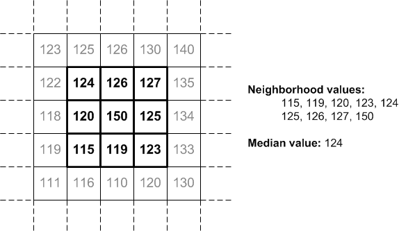
The Median filter is normally used to reduce noise in an image, and can often do a better job of preserving detail and edges in an image than the Mean filter. Like the Mean filter, this filter considers each pixel in the image in turn and looks at its nearby neighbors to decide whether or not it is representative of its surroundings. However, instead of simply replacing the pixel value with the mean of neighboring pixel values, it replaces it with the median of those values. Median filters are particularly useful for removing random intensity spikes that often occur in images captured in microscopes. The following illustration shows how this filter works. The median is calculated by first sorting all the pixel values from the surrounding neighborhood, in this case a 3 by 3 square, into numerical order and then replacing the pixel being considered with the middle pixel value. Median filter
As shown in the illustration, the central pixel value of 150 is not representative of the surrounding pixels and is replaced with the median value of 124. You should note that using larger neighborhoods will produce more severe smoothing. By calculating the median value of a neighborhood rather than the mean, the Median filter has two main advantages over the Mean filter:
However, the Median filter is sometimes not as subjectively good at dealing with large amounts of Gaussian noise as the Mean filter. It is also relatively complex to compute. |
Kernel shape and size |
| Minimum | Replaces each pixel in the image with the smallest pixel value in that pixel’s neighborhood. This grayscale erosion can help reduce salt noise. | Kernel shape and size
Mode |
| Non-Local Means* | Smoothes images by taking a mean of all pixels, weighted by how similar the pixels are to the target pixel.
Unlike the Mean filter, which takes the mean value of a group of pixels surrounding a target pixel to smooth an image, the Non-Local Means filter takes the mean of all pixels in the image, weighted by how similar they are to the target pixel. Applying this filter can result in greater post-filtering clarity with minimal loss of detail when compared with mean filtering. In many cases, the Non-Local Means or Bilateral filter should be your first choice for smoothing noisy images. You should note that non-local means filtering works most effectively if the noise present in the data is white noise, in which case most features present in the image will be preserved, even small and thin ones. References |
Kernel size
Smoothing Rician noise |
| Percentile | Percentile filtering is a well known non-linear technique for filtering images in which each pixel in the image is replaced by the value of that point in the histogram of its neighbour pixels that corresponds with a selected percentile. Percentile filtering includes minimum and maximum filtering (grey-value erosion and dilation) and median filtering. It is very suitable for background estimation and removal of outliers without degrading the image.
Note The median filter corresponds to the case where the percentile selected is 50. |
Kernel shape and size
Percentile value |
| Rank | Is a non-linear local filter that proceeds by ordering the pixels in a neighborhood and selecting a given ranked entry. | Kernel shape and size
Rank value |
| Tv_bregman | Performs total-variation denoising using a split-Bregman optimization. Total-variation denoising minimizes the total variation of an image, which can be roughly described as the integral of the norm of the image gradient.
Refer to http://en.wikipedia.org/wiki/Total_variation_denoising for more information about the principle of total-variation denoising. |
Weight
Max iteration Isotropic |
| Tv_chambolle | Performs total-variation denoising on n-dimensional images.
Note The code for the Tv_chambolle filter is an implementation of the algorithm of Rudin, Fatemi and Osher that was proposed by Chambolle in An algorithm for total variation minimization and applications, Journal of Mathematical Imaging and Vision, Springer, 2004, 20, 89-97. |
Weight
Max iteration |
| Wavelet | Performs a wavelet transform, using the selected wavelet function, which is characterized by a width parameter and length parameter. | Wavelet
Mode |
* Available only for Dragonfly 3D World ZEISS edition. Contact Comet Technologies Canada Inc. for information about the availability of this version of Dragonfly.