Reconstructing Cone-Beam Projections
Dragonfly's CT Reconstruction module includes the bench-marked algorithms for reconstructing 2D cone-beam projection data into 3D volumes, as well as iterative methods and pre-processing to improve image quality. In addition, geometry readers are provided for commercial CT scanners from Nikon, SkyScan, KA Imaging, North Star Imaging, GE, and other leading manufacturers.
Choose Workflows > CT Reconstruction on the menu bar to open the CT Reconstruction dialog. Then choose Cone Beam as the Beam type to access the reconstruction algorithms and pre-processing options for reconstructing cone-beam projections, as shown below.
CT Reconstruction dialog for cone-beam projections

The following settings and parameters are available in Dragonfly's CT Reconstruction module for reconstructing cone-beam projection data.
The options in the Input image box, shown below, let you choose the projection dataset that you want to reconstruct and a reconstruction package.
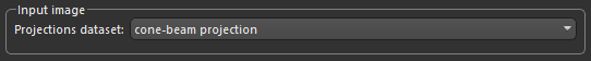
Projections dataset… Lets you choose the projection dataset that you want to reconstruct.
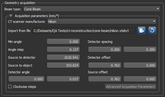
The options in the Geometry Acquisition parameters box, shown below, let you choose a beam type, import the acquisition parameters from a text file, or manually enter the geometry.
Geometry acquisition parameters
| Item | Description |
|---|---|
| Beam type | Lets you choose the beam type— Cone Beam or Parallel Beam — for tomographic data processing and image reconstruction. |
| Acquisition parameters | |
| CT scanner manufacturer | Lets you choose the device manufacturer of the CT system used to acquire the projection dataset. |
| Import from file |
Lets you choose the metadata file(s) that contains the acquisition parameters. The list of files is automatically filtered based on the device manufacturer as follows:
*.xtekct… For datasets acquired with Nikon CT systems.
Note If the metadata file is not available, you can enter the acquisition parameters manually, as described below. |
| Min angle | Is the minimum angle, in the indicated unit. |
| Angle step | Is the angle step, in the indicated unit. |
| Source to detector | Is the source to detector distance, in the indicated unit. |
| Source to object | Is the source to object distance, in the indicated unit. |
| Detector angle | Is the detector angle ranges from in-plane to out-of-plane, in the indicated unit. |
| Detector spacing | Is the detector spacing along the X and Y axes, in the indicated unit. |
| Detector offset | Is the detector offsets along the X and Y axes, in the indicated unit. |
| Source offset | Is the source offset along the X and Y axes, in the indicated units. |
| Clockwise steps | Lets you choose between clockwise and counter-clockwise steps. |
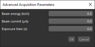
| Advanced Acquisition Parameters |
Opens the Advance Acquisition Parameters dialog, shown below. You can enter beam energy, beam current, and exposure time.
Note The advanced acquisition parameters are not used in this version of Dragonfly. |
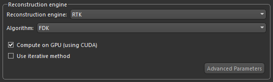
The options in the Reconstruction engine box let you choose a reconstruction engine, algorithm, and other parameters.
Reconstruction parameters
| Parameter | Description |
|---|---|
| Reconstruction engine |
Lets you choose a reconstruction engine.
RTK… Is an open-source software for fast circular cone-beam CT reconstruction based on the Insight Toolkit (ITK). Go to https://www.openrtk.org/ for more information about RTK. |
| Algorithm |
Lets you choose an algorithm.
FDK… The bench-marked Feldkamp-David-Kress (FDK) algorithm is a filtered back-projection algorithm that applies a filter in the frequency domain before back-projecting the projection images. Reference SART… Is an implementation of the Simultaneous Algebraic Reconstruction Technique (SART) iterative algorithm. You can choose a back-projection method for SART. Reference |
|
Compute on GPU (using CUDA) |
Lets you accelerate time-consuming reconstructions by computing on GPU. You should note that computing on GPU is required when using iterative methods for the FDK algorithm. |
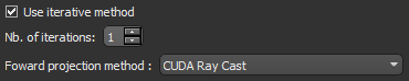
| Use iterative method |
Lets you choose a forward projection method — CUDA Ray Cast or Joseph — for iteration and the number of iterations.
|
| Advanced Parameters |
Opens the Advanced Reconstruction Parameters dialog, shown below.
Filtering… Lets you choose a filter and the filter settings for the reconstruction (see Filters). The quality of reconstructed images can be limited by several factors that result in poor spatial resolution, low contrast, and high noise levels. However, filtering can compensate for loss of detail in an image while reducing high-frequency noise. The filter chosen for a given image reconstruction task is mainly a compromise between the reduction of noise and the preservation of detail or contrast of the reproduced image. You should note that the Ramlak and Shepp-Logan filters are high pass filters that retain edges, while the Cosine, Hamming, and Hann filters are band pass filters. They are usually used to smooth images and remove extra edges from the image. Frequency cut… Lets you set cut-off frequency of the selected filter. A value of '0' will disable the filter. The value of the cut-off frequency determines how the filter will affect both image noise and resolution. A high cut-off frequency will improve the spatial resolution and detail, but the image may remain noisy. A low cut-off frequency will increase smoothing, but may degrade image contrast in the final reconstruction. Truncation padding… This parameter sets the amount of padding — '0' means no padding, '0.5' means padding with 50% more data, while the max value of '1' results in 100% padding. |
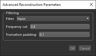
The following filters, which are applied to data in the frequency domain, are available in the Filter drop-down menu. You must set 'Frequency cut' to a value greater than 0 to enable filtering.
| Filter | Description |
|---|---|
| Cosine | The Cosine filter is obtained by multiplying the Ramlak filter by a cosine function. The advantage of the Cosine filter is that it reduces image noise. A disadvantage is that it does not preserve edges in the image. |
| Hamming | The low pass Hamming filter provides a high degree of smoothing. The only difference with the Hann filter is on the amplitude at the cut-off frequency. |
| Hann | The Hann ('Hanning') filter is a relatively simple low-pass filter that is very effective in reducing image noise. However, it often does not preserve edges well. |
| Ramlak | The Ramlak filter is a high−pass filter that blocks out low frequencies, which can cause blurring. If there are areas in the image where the signal changes rapidly a high−pass filter sharpens the edges and gives better contrast. A disadvantage of Ramlak and other high−pass filters is that they let pass high frequencies and as a consequence also noise. |
| Shepp-Logan | The Shepp-Logan filter belongs to the family of low pass filters and produces the least smoothing and has the highest resolution. |
Opens the CT Rotation Finder dialog, in which you can choose from a number of algorithms to find the rotation center offset for reconstructing cone-beam and parallel-beam projections (see CT Rotation Finder).
Opens the CT Rotation Finder dialog, in which you can find the optimal tilt angle, as well as the rotation center offset (see CT Tilt Angle Finder).
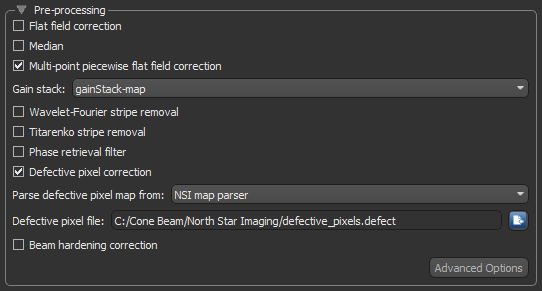
The pre-processing options let you choose to apply flat field corrections, median filtering, stripe removal, and other corrections to improve reconstructed image quality. Examples of filtering to remove ring artifacts correct defective pixels are shown in the images below.
No pre-processing (left), multi-point piecewise flat field correction (center) and with defective pixel correction (right)

Note Data courtesy of Pratt & Whitney Canada.
The following pre-processing options are available to improve reconstructed image quality.
Pre-processing options
| Option | Description |
|---|---|
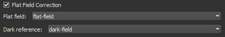
| Flat field correction |
Applies a linear calibration with flat field and dark field images to normalize projection data and remove ring artifacts. These artifacts can be caused by a variation in the pixel-to-pixel sensitivity of the detector and can also occur as a function of acquisition time. These artifacts can be seen in the sinogram of the sample.
Flat field… Lets you select the flat-field image taken with the X-ray beam turned on, but without the sample. Fixed pattern noise is removed with the assumption that the detector response did not change over the CT scan time. Dark reference… Lets you select the dark-field image taken before the X-ray beam was turned on. |
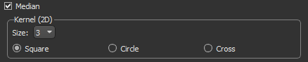
| Median |
Applies median filtering, at a selected kernel size and shape, to help smooth noisy data.
Note Median filtering is often used in conjunction with flat field correction, which normalizes projection data and removes ring artifacts. You should also note that median filtering not only removes noise, but can also remove image features. You need to be careful with selecting the kernel size. |
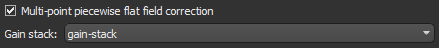
| Multi-point piecewise flat field correction |
Similar to flat field correction, but uses a multi-point image ('gain-stack') taken by changing the current at a constant step. The 'gain-stack' usually includes a flat field image and dark reference, as well as multiple steps between the flat field image and dark reference, to correct non-uniform backgrounds.
|
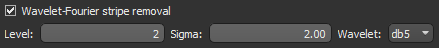
| Wavelet-Fourier stripe removal |
Removes horizontal and vertical stripes from the sinogram using the wavelet-Fourier based method.
Level… Lets you set the number of discrete wavelet transform levels. Sigma… Lets you set the damping factor in Fourier space. Wavelet… Lets you select a wavelet filter — 'db5', 'haar', or 'sym5'. In most cases, the default wavelet 'db5' provides the best results. Note In cases in which stripes are narrow, you can set 'Level' and 'Sigma' to low values. You should increase these parameters for broader or distorted stripes. Reference |
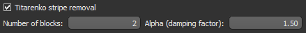
| Titarenko stripe removal |
Removes horizontal stripes and ring artifacts from the sinogram using Titarenko’s approach.
The adjustable parameters available for the Titarenko stripe removal filter include 'Number of blocks' and 'Alpha (damping factor)'. You may need to try different settings to achieve the best results. Reference |
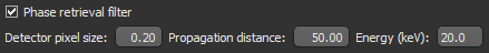
| Phase retrieval filter |
Used mostly for biological samples to perform a single-step phase retrieval from phase-contrasted environments.
Detector pixel size… Is the detector pixel size, which should be the same as detector spacing. The unit is the same as shown in the Geometry acquisition box. Propagation distance… Is the distance between the object and the detector. The unit is the same as shown in the Geometry acquisition box. Energy… Is the beam energy, in keV. Reference |
| Defective pixel correction |
Corrects defective pixels identified by a defective pixel map by averaging neighboring pixels. Defective pixels can sometimes be seen as straight vertical lines on the sinogram. You should note that this filter is often applied in conjunction with multi-point piecewise flat field correction.
Parse defective pixel map from… Lets you choose a North Star Imaging defective pixel map (if your data was acquired with a North Star CT system) or an image or region of interest defective pixel map. You can create a defective pixel map from the sinogram by applying a threshold to select and label defective pixels (see Creating Threshold Segmentations). Defective pixels are typically low intensity. Defective pixel file… Lets you choose the required file. |
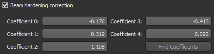
| Beam hardening correction |
Corrects beam hardening effects using coefficients of the projection. Each coefficient is to the power of 'x', where x is the coefficient number. For example, Coefficient 1 is to the power of 1, which is the projection itself.
Note The option to automatically find the coefficients in not available in this version of Dragonfly. |
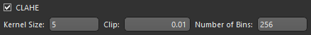
| CLAHE |
A variant of adaptive histogram equalization, contrast limited adaptive histogram equalization (CLAHE) improves local contrast and enhances the definitions of edges in each region of an image (see Contrast Adjustment Filters).
Selectable parameters include 'kernel size', 'clip', and 'number of bins'. |
| Advanced Options |
Opens the Advanced Pre-Preprocessing Filters dialog, shown below.
When Log is checked, the intensity of the projection will be inverted for filtering. This default setting is required when the background is bright and the scanned object is dark, as shown below.
If the background of the projection is already dark and the scanned object is bright, then you should uncheck Log. |
Lets you compute previews at the selected settings, as well as import the settings from a selected preview.
Preview options
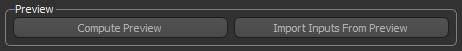
Compute Preview… Click this button to generate a one-slice preview using the selected settings.
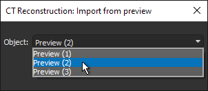
Import Inputs from Preview… Click this button to open the Import from Preview dialog. You can select any preview to reload the selected settings.
Lets you reconstruct projections at the selected settings.
Reconstruction options
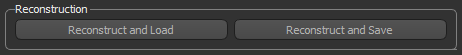
Reconstruct and Load… Click this button to reconstruct the selected dataset and then load the computed reconstruction into Dragonfly.
Reconstruct and Save… Click this button to reconstruct and save the selected dataset. You may need to do this if your system memory is not sufficient for loading the reconstructed dataset.
Refer to the following instructions for information about reconstructing cone-beam projections acquired from Nikon, SkyScan, North Star, KA Imaging, YXLON, GE and other CT scanner manufacturers.
- Load your cone-beam projection images (see Importing Image Files).
You will also need to load your flat field correction images or 'gain-stack' images for multi-point piecewise flat field correction if you plan to apply these pre-processing corrections to improve image quality (see Pre-Processing).
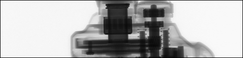
- Make sure that the projection image stack is oriented in the X-Y plane, as shown below.

Note If required, you can invert the X, Y, or Z axis or apply an axis transformation to re-orient the dataset (see Inverting Datasets).
- Choose Workflows > CT Reconstruction on the menu bar.
The CT Reconstruction dialog appears.
- Select your projection dataset in the Projections dataset drop-down menu.
- Select Cone Beam in the Beam type drop-down menu.
The acquisition parameters, reconstruction engine options, and pre-processing options for cone-beam projection images appear in the dialog.
- Do one of the following:
- Choose the manufacturer of the CT scanning system used to acquire the data in the CT scanner manufacturer drop-down menu.
- Click the Import
 button.
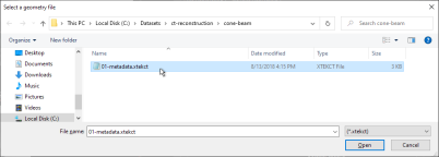
If you selected Nikon, SkyScan, KA Imaging, YXLON, or GE as the manufacturer, navigate to and open the file that contains the metadata for the loaded dataset in the Select a Geometry File dialog.
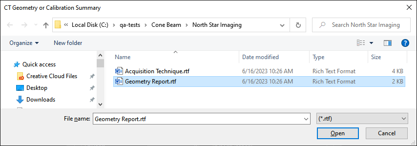
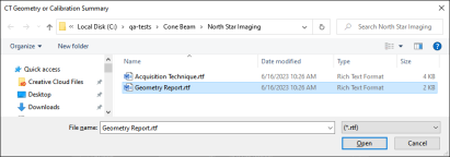
If you selected North Star Imaging as the manufacturer, navigate to and open the rich-text formatted file (*.rtf extension) that contains the geometry information for the loaded dataset in the CT Acquisition Technique Sheet dialog. You will also need to load the RTF file that contains the geometry or calibration summary for the loaded dataset in the CT Geometry or Calibration Summary dialog.
- Enter the geometry information manually (see Geometry Acquisition).
- Choose a reconstruction engine, algorithm, and other required parameters in the Reconstruction engine box (see Reconstruction Engine).
- If required, find the rotation center offset and/or tilt angle (see CT Rotation Finder and CT Tilt Angle Finder).
- Choose the required pre-processing corrections (see Pre-Processing).
Note By default, Log is selected in the Advanced Pre-Processing Filters dialog, as shown below. This setting is required whenever the background of the projection images is bright and the scanned object is dark.
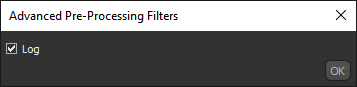
To change this setting, click the Advanced Options button in the Pre-Processing box and then uncheck Log.
- Click the Compute Preview button and then review of results of the one-slice reconstruction.
- If the result is acceptable, continue to the next step.
- If the result is unacceptable, modify the reconstruction parameters and/or pre-processing options and then generate another preview.
Note You can load the settings of the best preview by clicking the Import Inputs from Preview button and then selecting the best preview in the Import from Preview dialog.
- Do one of the following:
- Click the Reconstruct and Load button to compute and load the reconstructed dataset.
Note If this option exceeds your system's memory, you can choose to reconstruct and save or you can crop the projection dataset (see Cropping Datasets). If you choose to crop the dataset, you must remove an equal number of slices from the top and bottom of the projection (Y-axis). After cropping, you can choose the new dataset in the Projections dataset drop-down menu.
- Click the Reconstruct and Save button to compute and save the reconstruction as multiple TIFF files. You will need to choose a location for the reconstructed dataset in the Export Reconstruction to File dialog.
- Click the Reconstruct and Load button to compute and load the reconstructed dataset.